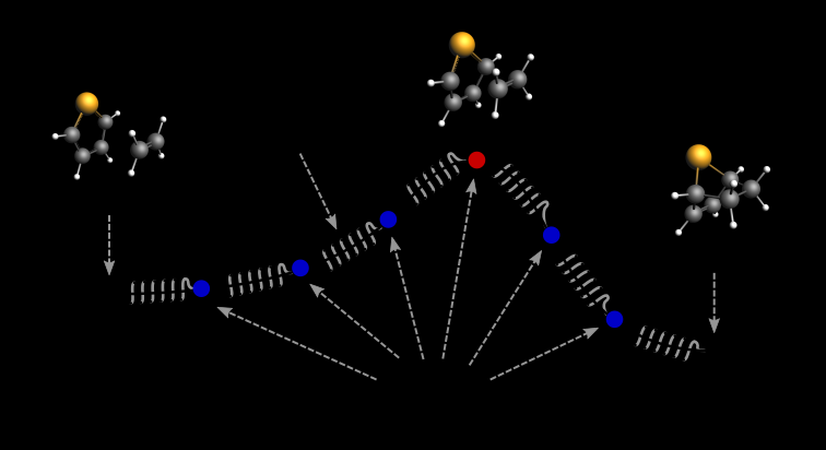
NEB calculations parallelized over images — GPAW (dtu.dk)
1 初始化
from ase import Atoms
from ase.build import add_adsorbate
from ase.visualize import view
from ase.constraints import FixAtoms
from ase.optimize import QuasiNewton
from ase.io import write,read
from ase.calculators.emt import EMT
from gpaw import GPAW, PW
from ase.calculators.dftd3 import DFTD3 # van der Waals
import numpy as np
from ase.neb import NEB
import matplotlib.pyplot as plt
from ase.optimize.sciopt import SciPyFminCG # conjugate gradient

## Find the initial and final states for the reaction.
Mg2S2 = Atoms('Mg2S2',[[0,0,0],[3.7,0,0],[1.85,1.85,0],[1.85,-1.85,0]]) # Mg2S2 from Materials Project
## Set up a (4 x 4) two layer slab of Cu:
slab = read('BiN4.cif') # BiN4 from the article
## slab.set_pbc((1, 1, 1)) # Set periodic boundary conditions. (1,1,0) means periodic in x and y, but not in z.
add_adsorbate(slab,Mg2S2,height=4.0,position=(2.383, 5.455)) # height means the distance between the adsorbate and the surface. position means the x-y position of the adsorbate, 'fcc' means the position of the (0,0,0) with shift to fcc postion
## slab.center(vacuum=10, axis=2) # set a 20 A vacuum along the z-axis
view(slab)
1.1 优化初始结构
## The forces of the atoms are the dE/dx of the atoms.
## default ecut of PW is 340 eV
mask = [atom.symbol == 'C' for atom in slab]
slab.set_constraint(FixAtoms(mask=mask))
slab.calc = GPAW(xc='PBE', mode=PW(400)) # default kpts is only the gamma point.
## Relax the structure
relax = QuasiNewton(slab) # Structure optimization using the QuasiNewton method (BFGSLineSearch)
relax.run(fmax=0.05) # fmax is the maximum force = 0.05 eV/Ang
view(slab)
write('N2.traj',slab)
1.2 优化最终结构
## Now the final state.
## Move the second N atom to a neighboring hollow site:
## slab[-1].position[0] means the x-coordinate of the last N atom
## slab[-1].position[1] means the y-coordinate of the last N atom
## slab.cell[0, 0] means the x-dimension of the slab
slab[-1].position[0] = slab[-2].position[0] + 0.25 * slab.cell[0, 0] # shift N atom to the right by 0.25 times the x-dimension of the slab
slab[-1].position[1] = slab[-2].position[1]
## and relax.
relax.run()
view(slab)
write('2N.traj', slab)
2 初始化路径图像
## Read the previous configurations
initial = read('N2.traj')
final = read('2N.traj')

##  Make 9 images (note the use of copy)
configs = [initial.copy() for i in range(8)] + [final] # 8 of initial and 1 of final images

## As before, fix the Cu atoms
constraint = FixAtoms(mask=[atom.symbol != 'N' for atom in initial])
for config in configs:
    config.calc = EMT() # config the calculator of every image, only the internal images (not the endpoints) need have calculators attached.
    config.set_constraint(constraint) # set the constraint of every image
3 用NEB法进行优化求解
## Make the NEB object, interpolate to guess the intermediate steps
band = NEB(configs)
band.interpolate() # linear interpolation
relax = QuasiNewton(band, trajectory='N2Cu.traj') # Structure optimization using the QuasiNewton method (FIRE)
## Do the calculation
relax.run() # default fmax=0.05
4 绘制路径图像
e0 = initial.get_potential_energy()
E = [config.get_potential_energy() - e0 for config in configs]
plt.plot(E)